The Vicor On-Line Simulator provides a means to accurately simulate the electrical and thermal behavior of Vicor products. The user can define the operating and environmental conditions of the subject Vicor product. In addition to setting the basic Line and Load conditions, the user can also adjust input and output impedance and filters conditions. A variety of simulation types can be performed over a defined simulation period. Simulation result charts and tables accurately show product performance based on the user settings provided.
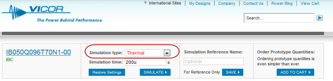
Products to be simulated are presented in what is known as a Reference Design for the product in question. For example, the following is the Reference Design for an Intermediate Bus Converter, IBC, intended for a Thermal Simulation:
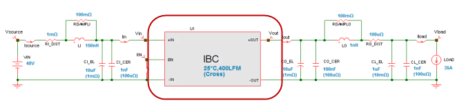
Reference Designs are typically divided into 3 sections; Input, Product and Output.
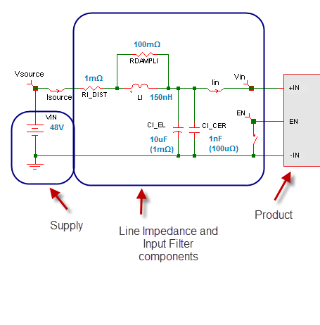
The Input section comprises of the Supply or Source as well as a set of components to represent Line Impedance, Input Filtering and Input Holdup Capacitance:
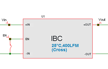
The Product itself is usually at the center of the Reference Design:
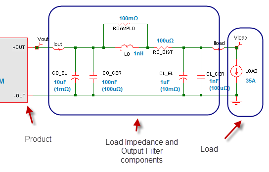
The Output section comprises of the Load as well as a set of components to represent Load Line Impedance, Output Filtering and Output Holdup Capacitance:
There can be multiple simulation types available for each Reference Design. They are selected from a drop-down list at the top of the page:
The simulation types for an IBC are:
| Simulation | Description | Results |
|---|---|---|
| Thermal | Simulates the electrical performance at steady state electrical conditions and with a user defined thermal environment; ambient air-temperature, airflow and airflow direction. | A table with power loss, efficiency and the predicted operating temperature of the unit. Also charts with input and output current and voltage waveforms. |
| Steady-State | Simulates the electrical performance at steady state electrical conditions and at a user defined fixed operating temperature. | A table with power loss, efficiency etc. Also charts with input and output current and voltage waveforms. |
| Vin Start-up | Simulates the behavior of the unit on applying Vin. The Load Mode can be set in Constant Current, Constant Resistance or Constant Power Mode. | Charts showing Vin startup, Vout Start and Vout Start delay, Inrush Current etc. |
| Vin Step | To simulate an input transient by changing Vin from a starting value to an ending value at a user defined ramp-rate in V/us. The starting value can be greater than or less than the ending value. Either value can be inside or outside the operating range of the product. If either value is outside the operating range of the units, then the unit will behave accordingly. | Charts show Vin step, Iin change, Vout change and Iout change. |
| Load Step | To simulate an load transient by changing the load from a starting value to an ending value at a user defined ramp-rate in A/us. The starting value can be greater than or less than the ending value. Either value can be inside or outside the operating range of the product. If either value is outside the operating range of the units, then the unit will behave accordingly. | Charts show Load step, Iin change, Vout change and Iout change. |
| EN Startup | To simulate the startup behavior of the unit when Vin is already applied and the unit goes from a disabled to an enable state by changing the EN pin to the appropriate level based on the operating logic of the Enable Pin. | Charts show the En pin change and the corresponding change in input and output conditions. |
| EN Shutdown | To simulate the shutdown behavior of the unit when Vin is already applied and the unit goes from a enabled to a disabled state by changing the EN pin to the appropriate level based on the operating logic of the Enable Pin. | Charts show the En pin change and the corresponding change in input and output conditions. |
The Simulation Time, as the name suggests, allows the user to adjust the amount of time over which a simulation occurs. If too low or too high a value is chosen the value entered will be overridden by the default minimum or maximum value.

Component values on the schematic can be changed either by clicking on the component itself or by clicking on the component value:
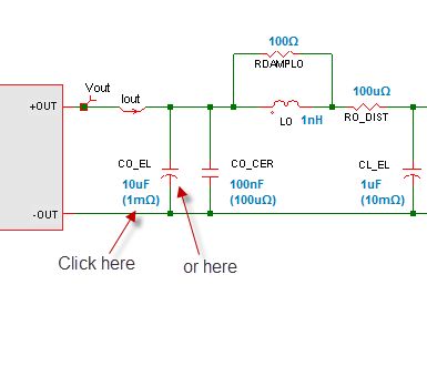
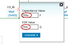
On clicking either the component or its value, a dialog box appears next to the component, where the new value can be entered.
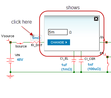
For example, click next to a resistor
Component values are entered along with SI unit prefixes. The more common prefixes used in the simulator are:
| Prefix | Name | Scientific Notation | Standard Notation |
|---|---|---|---|
| M | Mega | 1E6 | 1,000,000 |
| k | kilo | 1E3 | 1,000 |
| m | milli | 1E-3 | 0.001 |
| u | micro | 1E-6 | 0.000001 |
| n | nano | 1E-9 | 0.000000001 |
The units themselves are shown next to the entry boxes. So, in the example, entering "5m" is all that's needed to set the resistor in question to 0.005Ω.
Components such as resistors will only have have one attribute associated with them. In the case of a resistor, it will be the resistor value in Ohms. Other components such as capacitors will have two or more attributes associated with them. A capacitor will have its value in Farads as well as an ESR value in Ohms.
For example, a 10μF capacitor which has a 1mΩ ESR.
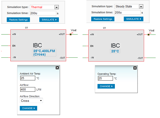
In the Reference Design for both the Thermal Simulation as well as the Steady-State Simulation, the thermal conditions of the product itself can be changed by clicking on the unit itself or its thermal values. In this respect, changing the thermal properties of the unit is an identical process to changing the values of any component in the Reference Design. In the following, Thermal Simulation is shown on the left and Steady-State Simulation is shown on the right.
All the schematic values can be restored to their default value for the simulation
and part number in question by clicking on the  button.
To execute the simulation, click the  button:

As the simulation is running, the Reference Design is replaced by the following:

When the Simulation has run, the Reference Design is shown once again, and is followed by the Simulation results.
If the Simulation was either Steady-State or Thermal, then following the schematic a table is shown as follows:
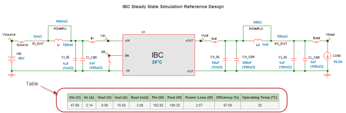
This contains a set of values, calculated by the Simulator, that show Power Loss and Efficiency at the Line, Load and Thermal Conditions specified. In the case of a Thermal Simulation the actual Temperature of the product is also shown which is based on the Electrical and Thermal conditions.
For example, conducting the following simulation with a unit operating from a 44V supply and with a 17A load, in 44⋅C ambient air with 400LFM across the product results in the unit operating at 53°C and at an efficiency of 97.89%.

Following the efficiency/power loss and temperature table are the result waveforms. Typically the waveforms are shown in multiple charts with two or more waveforms per chart. Individually each chart can be selected by clicking anywhere on the chart.
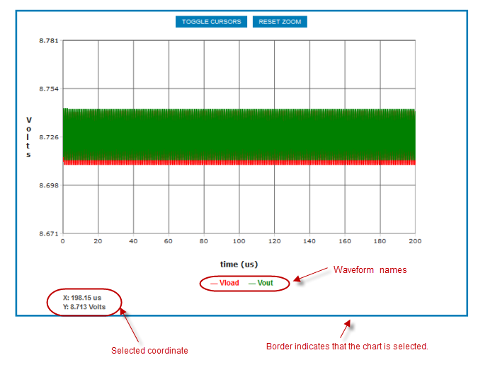
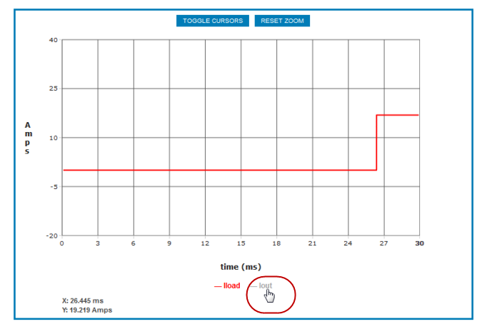
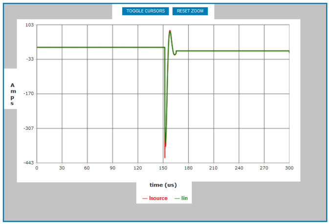
Waveform names are shown below the chart and waveforms can be turned on and off by clicking on the waveform names themselves. In the following example, Iload waveform is shown in red and Iout can be added by clicking on the waveform name:
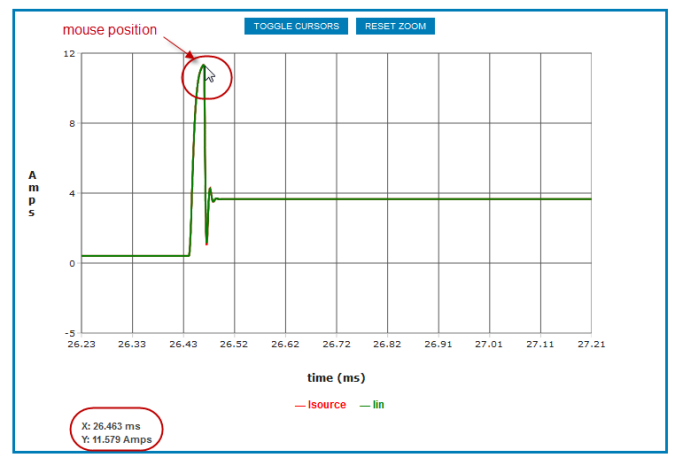
Moving the mouse along a wavform will cause an X,Y tip to show the X,Y value of the waveform at the pointer position. For example the pointer position in the following waveform is shown at the peak of the signal. The X and Y values corresponding to that position are shown below the waveform. In the example, the X value is 26.463ms after the start of the simulation and the Yvalue is 11.579 Amps. In this case, that is a convenient way of measuring peak Inrush Current.
The waveforms shown typically contain much more datapoints than are visible on the screen. A zoom capability is made available to magnify any area of the waveform.
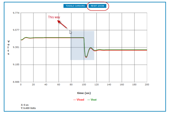
To zoom, drag across the area of interest in the direction shown as follows:
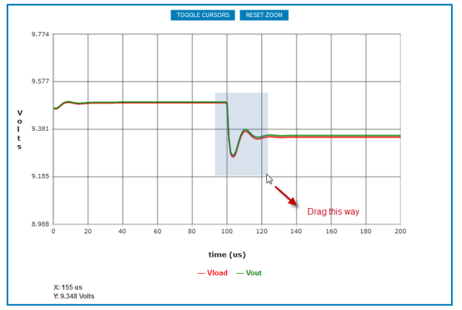
The zoom area can be a rectangle of any size. Following the zoom, the chart in question will be resized and rescaled to occupy the zoomed rectangle. All other charts will also be zoomed to the same degree in the X-axis. In other words, the other charts will be zoomed to show the same slice of time as the subject chart. The Y-axis of the other charts will be not change.
The following shows the previous chart after zooming:
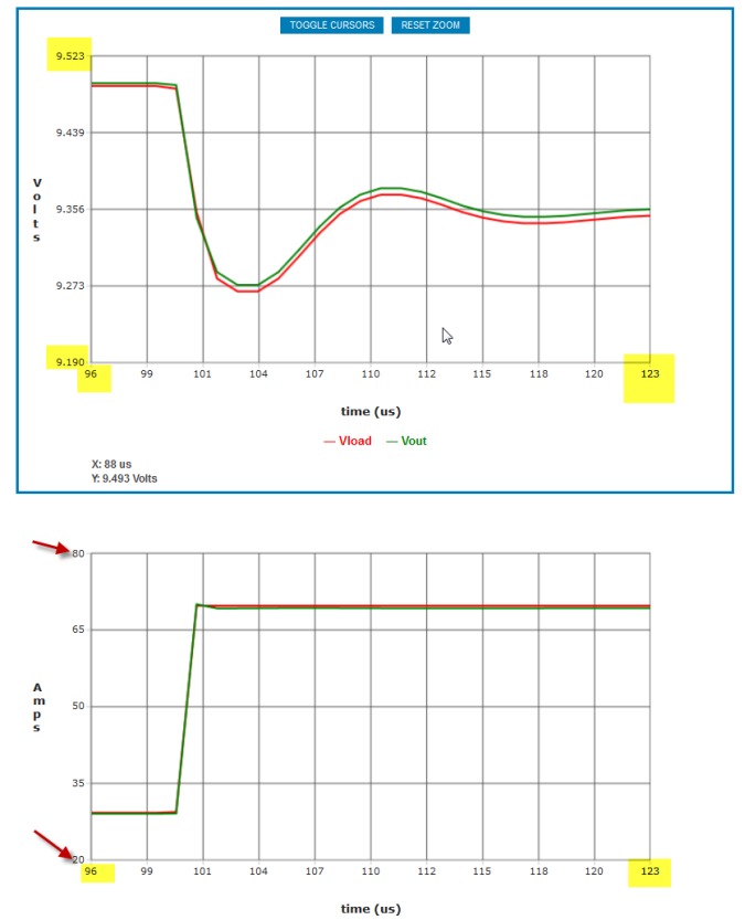
Further zooming can be done in the same fashion.
There are two ways to Reset the zoom or to show the original level of detail..Either
click on the  button or drag across the chart in the direction
shown:
button or drag across the chart in the direction
shown:
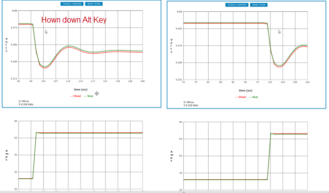
After zoom, to pan or shift the the wavform in any direction, hold down the Alt Key and with the pointer anywhere on the chart, drag the waveform as needed.
The waveform view capability includes a set of cursors that are used to measure
X-Y differences. The cursors can be toggled on and off using the  button
above the selected chart. The cursors appear as 4 dashed lines indicated by
the red arrows as follows:
button
above the selected chart. The cursors appear as 4 dashed lines indicated by
the red arrows as follows:
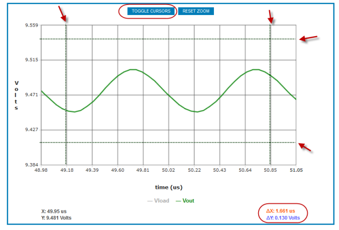
On the bottom right hand corner of the waveform the delta X and Y values are shown. Delta X is typically based on the time difference between the two vertical cursors and Delta Y is typically based on the voltage or current difference between the two horizontal cursors.
The cursors can be dragged to the required position for a specific measurement or measurements. For example to measure the period and peak to peak amplitude of the sinuosidal output of an IBC, drag the cursors as follows:
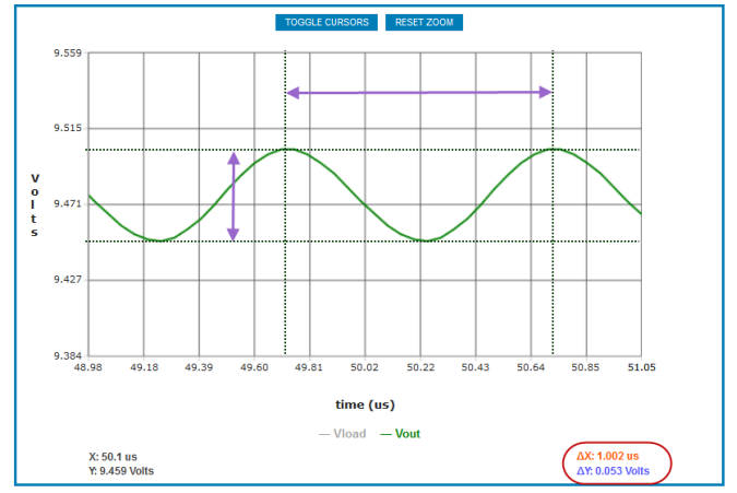
In the example, the peak to peak voltage is 53mV and the period 1.002us.
To drag, or move a chart, to another area of the browser window, click in any part of the shaded area of the chart and drag as needed.
A Store and Compare capability is also made available in order to compare simulation results. For example, to understand the effect of an increased slew rate input volatge step and the output voltage response, the waveforms associated with the initial simulation can be super-imposed with the waveforms associated with the subsequent simulation.
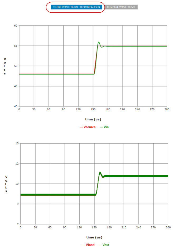
For example, performing the initial simulation, with the input supply stepping
from 48V to 55V at 1V/us produces the following the results. These results can
be stored for later comparison purposes using the  button.
After a subsequent simulation, using a faster slewrate, the original waveforms
can be added to the new charts using the ![]() button.
button.

In this case, the chart will show 4 waveforms; the two most recent as well as the two that were stored. Any of these waveforms can be shown or hidden by clicking on the legends below the chart as normal.
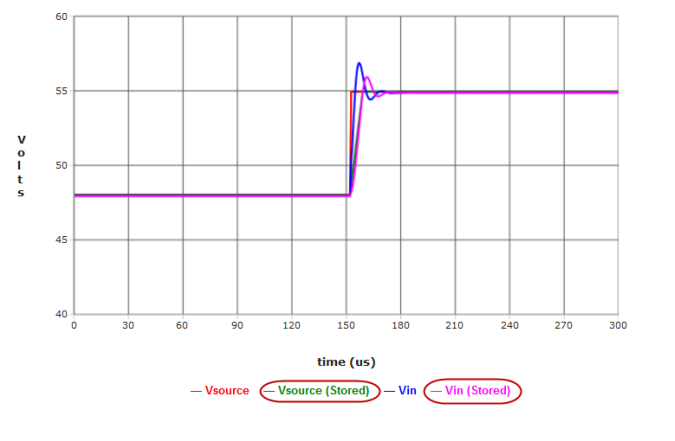
So, in the example, turning off Vload and Vload (Stored), then zooming and using the cursors, it can be seen that output voltage overshoot is 246mV greater when the supply voltage changes at 10V/us instead of 1V/us.

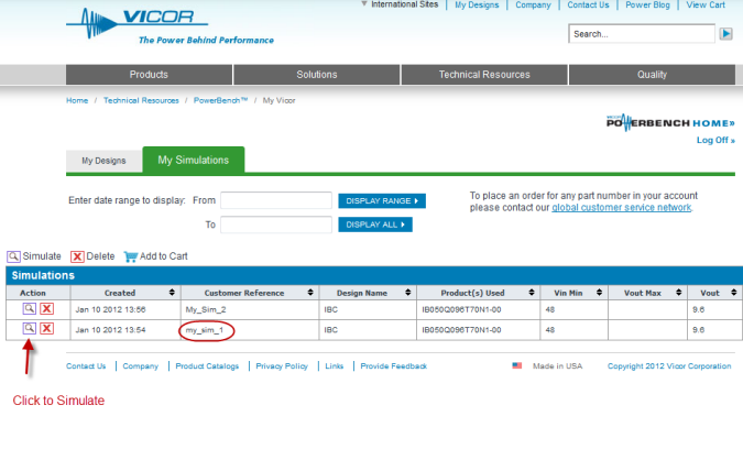
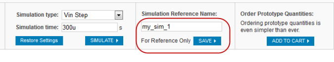
Simulations can be saved for later use by assigning a unique name to the simulation
performed and clicking on the  button:
In order to save simulations, it is necessary to have an account and be logged on to the Vicor Design Center. If you are not already logged on, then the following logon screen is shown:
After saving the simulation, the following acknowledgement is shown:

Under My Simulations is a list of all saved simulations, any of which can be recalled by clicking on the icon in the Action column.